Multi-layer Perceptrons and Backpropagation

Part 3 of 3 in Foundations of AI
Introduction
Something clicked for me when I was actually running training loops during my final year project — not reading about training, but sitting there watching loss curves descend in a terminal. Training a neural network looks like magic from the outside. From the inside, it’s an optimisation problem. You have a network making predictions, you have a measure of how wrong those predictions are, and you have a systematic way of nudging every single weight in the right direction. That’s it. The sophistication is in making that nudge efficient across millions of parameters.
XOR has been a thread running through all three posts in this series. The perceptrons post showed why a single neuron can’t solve it — no straight line separates the 1s from the 0s. The activation functions post showed why non-linearity is the ingredient you need. This post is where XOR finally gets solved, with a network you can run yourself.
The goal
By the end of this article, you’ll understand:
- Why stacking layers with non-linear activations solves problems a single perceptron cannot.
- The structure of an MLP: input, hidden, and output layers.
- What loss functions are and when to use MSE versus cross-entropy.
- What gradient descent is actually doing.
- How backpropagation works — both why it’s needed and how it runs.
- How to implement all of this from scratch in NumPy and train an MLP on XOR.
Prerequisites
- Perceptrons — weighted inputs, the step function, and why XOR breaks a single neuron.
- Activation Functions — why non-linearity matters and the trade-offs between common choices.
- Basic Python (the code examples use NumPy).
Why stacking works
A single perceptron draws one straight line. XOR needs more than that — the 1s and 0s sit in opposite corners of a grid, and no single boundary separates them.
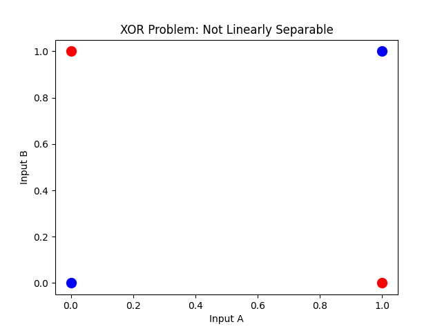
Marvin Minsky and Seymour Papert proved this formally in Perceptrons (MIT Press, 1969). Their proof that single-layer perceptrons cannot represent XOR contributed to a decade-long slowdown in neural network research — the so-called AI winter — until backpropagation revived the field in the 1980s.
Stack two layers and the picture changes. The first layer doesn’t try to solve the problem directly — it transforms the input into a new representation where the problem becomes linearly separable. The second layer then draws that final boundary.
Mathematically, instead of a single transformation:
You compose two:
Where:
- = activation functions at each layer
- = weight matrices
- = bias vectors
- = input vector
The critical point is the non-linear activation between layers. Without it, the composition collapses back into a single linear transformation — as the activation functions post showed, depth without non-linearity buys you nothing. With it, each layer reshapes the input space in a way the next layer can exploit.
Structure of a Multi-Layer Perceptron
An MLP has three types of layers:
- Input layer — receives the raw data. No computation; it just passes values through.
- Hidden layers — each neuron computes a weighted sum of its inputs, adds a bias, and applies a non-linear activation function. This is where features are extracted.
- Output layer — produces the final prediction. For binary classification, a single neuron with a sigmoid activation gives a probability between 0 and 1.
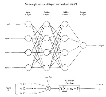
Per layer, the transformation is:
Where is the output of layer and is the output of the previous layer (or the raw input when ).
The hidden layers are a genuine black box. Their weights are discovered automatically during training rather than designed by hand, which creates an explainability problem that hasn’t been fully solved. If a neural network is recommending a mortgage decision or flagging someone in a legal context, “the hidden layers decided” is not an acceptable answer. For problems where full traceability matters, MLPs are sometimes set aside in favour of models whose decisions can be audited step by step.
Multi-class problems (classify this digit as 0–9) need an output that sums to one across all classes — a proper probability distribution. Softmax does that job. It takes a vector of raw scores (logits) and converts them into a vector of non-negative values that sum to 1:
For example, logits become approximately after softmax — a clear winner, but with quantified uncertainty across all classes. For binary classification like XOR, you don’t need softmax; a single sigmoid output is enough.
How MLPs learn
Training a neural network comes down to two things: figuring out how wrong the model is, and figuring out how each weight contributed to that wrongness. Loss functions handle the first. Gradient descent and backpropagation handle the second.
Loss functions
A loss function measures how wrong a prediction is, relative to the true label. The choice depends on what kind of prediction you’re making.
Mean Squared Error (MSE) is the natural choice for continuous outputs — predicting a house price, forecasting revenue, estimating a temperature reading. It penalises large errors more heavily than small ones:
Binary Cross-Entropy is the right choice for binary classification — spam or not spam, XOR’s 0 or 1. It measures how surprised the model should be by the correct label, given its predicted probability:
When the model predicts high confidence in the right answer, the loss is low. When it’s confidently wrong, the loss is large — and the penalty grows steeply.
Gradient descent
Once you have a loss value, the question is which direction to nudge the weights to make it smaller. Gradient descent answers that by computing the slope of the loss surface with respect to each parameter.
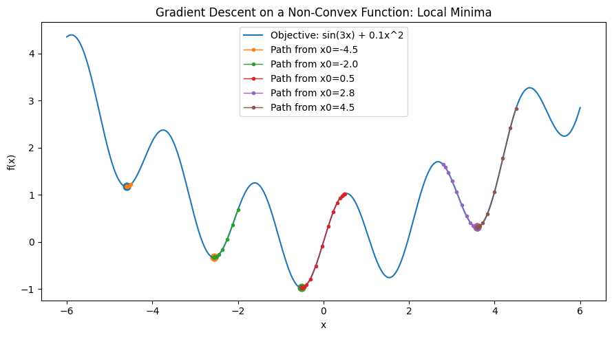
The gradient tells you: if I increase this weight slightly, does the loss go up or down? By stepping in the direction that decreases the loss, the model gradually improves. The size of each step is controlled by the learning rate — too large and you overshoot; too small and training takes forever.
Finding the global minimum is harder than it sounds. The loss surface has local minima, flat plateaus, and saddle points. In practice, gradient descent finds a solution that’s good enough rather than provably optimal, and various tricks (momentum, adaptive learning rates, random restarts) help it avoid the worst traps.
Standard gradient descent computes the loss and gradient across the entire dataset before taking a single step. That’s expensive for large datasets. Stochastic Gradient Descent (SGD) uses a single example, or a small random mini-batch, per update — noisier, but much faster to converge in practice. Most training runs use mini-batch SGD. For the XOR example here, the dataset has four examples and the distinction doesn’t matter — full-batch gradient descent is fine.
Backpropagation
Gradient descent tells you how far to nudge each weight. Backpropagation tells you what gradient to use for each weight across every layer. These two things are distinct, and getting them mixed up is a common source of confusion.
The purpose: blame propagation
Think of it this way. The network just made a prediction. It was wrong. Every weight in every layer contributed to that wrongness — some a lot, some barely at all. Backpropagation answers the question: how much of the blame does each weight deserve?
That blame is the gradient. A weight with a large gradient had a large effect on the error. A weight with a near-zero gradient barely mattered. Once you know the blame for each weight, gradient descent uses it to decide how far to nudge each one.
The mechanism: chain of consequences
Why can’t you just look at each weight directly? Because in a deep network, a weight in the first layer affects the output only through many intermediate steps. It influences its layer’s activations, which influence the next layer’s activations, which eventually influence the output and the loss.
The chain rule from calculus handles exactly this situation. When one quantity affects another through a sequence of steps, the total effect is the product of the small effects at each step. Backpropagation applies the chain rule systematically, working backwards from the output to the input.
The name is literal: gradients propagate backwards through the network, layer by layer.
The three stages
-
Forward pass — run the input through the network and store every intermediate value: the pre-activation sums, the activation outputs, and the final loss. These stored values are needed during the backward pass.
-
Backward pass — starting at the output layer, compute how each weight and bias contributed to the loss. Apply the chain rule at each layer, working backwards. The gradient at each layer depends on the gradient from the layer ahead of it and the stored intermediate values from the forward pass.
-
Gradient collection — by the end of the backward pass, every weight and bias has a gradient. One forward pass and one backward pass gives you everything needed for a gradient descent update across the entire network. This is what makes training deep networks computationally tractable; without it, you’d need a separate calculation for every parameter.
Solving XOR from scratch
The cleanest way to cement this is to implement it. The following trains a two-layer MLP on XOR using only NumPy — no frameworks, no .backward(), no magic. Forward pass, loss, backward pass, weight update, repeat.
Architecture:
- 2 inputs
- 4 hidden neurons with Leaky ReLU (consistent with the recommendation in the activation functions post)
- 1 output neuron with sigmoid (probability interpretation for binary classification)
- Binary cross-entropy loss
- Learning rate 0.1 over 5,000 epochs
import numpy as np

# --- Activation functions ---

def leaky_relu(z, alpha=0.01):
    return np.where(z >= 0, z, alpha * z)

def leaky_relu_grad(z, alpha=0.01):
    return np.where(z >= 0, 1.0, alpha)

def sigmoid(z):
    return 1 / (1 + np.exp(-z))

# --- XOR dataset ---

X = np.array([[0, 0], [0, 1], [1, 0], [1, 1]], dtype=float)
y = np.array([[0], [1], [1], [0]], dtype=float)

# --- Initialise weights ---

rng = np.random.default_rng(42)
W1 = rng.standard_normal((2, 4)) * 0.1   # 2 inputs  → 4 hidden neurons
b1 = np.zeros((1, 4))
W2 = rng.standard_normal((4, 1)) * 0.1   # 4 hidden  → 1 output neuron
b2 = np.zeros((1, 1))

lr = 0.1
epochs = 5000

for epoch in range(epochs):

    # Forward pass — store all intermediates
    z1 = X @ W1 + b1        # pre-activation, hidden layer
    a1 = leaky_relu(z1)     # activation, hidden layer
    z2 = a1 @ W2 + b2       # pre-activation, output layer
    a2 = sigmoid(z2)        # predicted probability

    # Loss — binary cross-entropy
    loss = -np.mean(
        y * np.log(a2 + 1e-8) + (1 - y) * np.log(1 - a2 + 1e-8)
    )

    # Backward pass — chain rule applied layer by layer

    # Output layer: combined BCE + sigmoid gradient simplifies to (a2 - y) / n
    dL_dz2 = (a2 - y) / len(y)

    dL_dW2 = a1.T @ dL_dz2
    dL_db2 = dL_dz2.sum(axis=0, keepdims=True)

    # Hidden layer: gradient flows back through W2, then through Leaky ReLU
    dL_da1 = dL_dz2 @ W2.T
    dL_dz1 = dL_da1 * leaky_relu_grad(z1)

    dL_dW1 = X.T @ dL_dz1
    dL_db1 = dL_dz1.sum(axis=0, keepdims=True)

    # Gradient descent update
    W2 -= lr * dL_dW2
    b2 -= lr * dL_db2
    W1 -= lr * dL_dW1
    b1 -= lr * dL_db1

# Final predictions
print("Predictions after training:")
for inputs, pred in zip(X.astype(int), a2.flatten()):
    print(f"  {inputs} → {pred:.4f}")
After 5,000 epochs the output looks something like this:
Predictions after training:
  [0 0] → 0.0312
  [0 1] → 0.9671
  [1 0] → 0.9669
  [1 1] → 0.0381
The network has converged on XOR — a single perceptron can’t do this. Two layers with non-linear activations can, and the backward pass is what taught them how.
A few things worth noting in the code:
The combined gradient for a sigmoid output with binary cross-entropy is (a2 - y) / n. That simplification comes from working through the chain rule for both operations together — the result is clean, and it’s worth knowing it rather than computing BCE and sigmoid gradients separately every time.
The hidden layer gradient chains through W2 first (dL_dz2 @ W2.T), then through the Leaky ReLU derivative. That’s the chain rule in action — the gradient of the loss with respect to the hidden layer activation equals the upstream gradient scaled by the local derivative.
The small constant 1e-8 inside the logarithms prevents numerical issues when a prediction is very close to 0 or 1. It’s a practical detail that doesn’t appear in the mathematics but matters in any real implementation.
Conclusion
This post covered the full stack from stacking layers to training them. MLPs solve what single perceptrons cannot, because composing non-linear transformations across layers creates flexible decision boundaries. Loss functions give you a measure of wrongness. Gradient descent uses the gradient of that loss to nudge each weight in the right direction. Backpropagation efficiently computes those gradients for every parameter in a single backward sweep — by propagating blame back through the network using the chain rule.
The from-scratch implementation is useful for understanding. Once you’ve written the backward pass by hand, what PyTorch and JAX do under the hood when you call .backward() stops being mysterious. In production, you’d use a framework rather than hand-rolling gradients — automatic differentiation handles arbitrary architectures correctly and efficiently. But having done it once, manually, you’re no longer taking it on faith.
The natural next step from MLPs is handling data with structure. Text is sequential — the order of words matters. Images are spatial — nearby pixels are related. MLPs treat every input feature as independent, which limits what they can do with these data types. Recurrent neural networks address sequences, and convolutional networks address spatial structure. I’ll get to both of those eventually.
Further Reading:
- Perceptrons — the first post in this series
- Activation Functions — the previous post in this series
- Learning Representations by Back-propagating Errors — Rumelhart, Hinton, Williams (1986) — the original backpropagation paper
- The Chain Rule — BBC Bitesize — a plain-English introduction to the calculus underpinning backpropagation
Part 3 of 3 in Foundations of AI