Activation Functions

Part 2 of 3 in Foundations of AI
Introduction
This post is part of the Foundations of AI series. In the previous article on perceptrons, I covered how a single neuron takes weighted inputs and fires a decision. Activation functions are what make that decision happen — and what determines how useful it is.
I wrote most of these posts during my final year of part-time university. I was studying a machine learning and artificial intelligence module that ran from ELIZA all the way through to ChatGPT and deepfakes — one of the best things I’ve done professionally. My final year project was building an AI chatbot for museum visitors to converse with about the Iliad and the Odyssey, which meant I spent a lot of time actually training models rather than just reading about them.
That timing mattered because AI was everywhere. Every newsletter, every LinkedIn post, every conference talk. Plenty of opinionated takes in both directions, but very few that explained the actual mechanics. Not “here’s why AI will save or destroy us”, but “here’s what actually happens inside the network.” That gap is what this series is trying to fill.
Activation functions are a good example of where standard documentation falls flat. Most articles assume prerequisite maths knowledge, or skip over it entirely, and land somewhere in the middle that isn’t much use to anyone. This post starts with the reason they exist, works through the trade-offs honestly, and ends with an actual opinion on what to reach for.
The goal
By the end of this article, readers will understand:
- Why non-linear activation functions exist — and what goes wrong without them.
- How the most common activation functions actually behave, not just what their equations look like.
- The key trade-offs between sigmoid, tanh, ReLU (Rectified Linear Unit), Leaky ReLU, ELU (Exponential Linear Unit), and Mish.
- What the vanishing gradient problem is — and why it is a real problem, not just a theoretical one.
- Which activation function I’d reach for in practice, and why.
Prerequisites
- Perceptrons — specifically how weighted inputs are summed and passed to an activation function.
- Basic Python (the code examples use NumPy and Matplotlib).
Why stacking layers without non-linearity does nothing
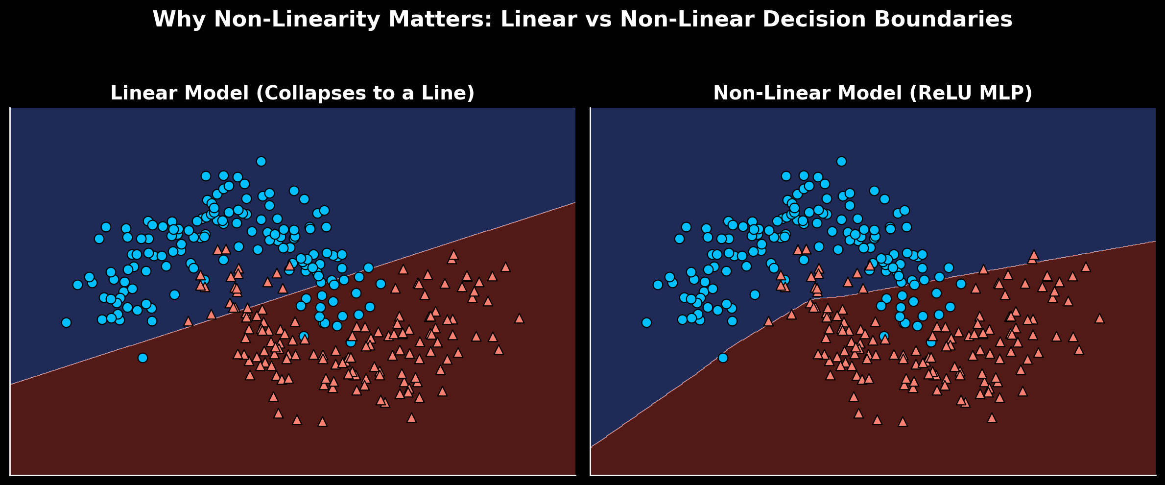
Here’s the core problem. If all you use are linear transformations, stacking layers doesn’t actually give you more expressive power — it all collapses back into a single transformation.
Imagine you’re an Eques during the reign of Nero, and a cushy administrative job has opened in Egypt. You climb the social ladder, do your military service, grease the palms of senators to eventually be considered for the role. Nero is famously corrupt, so all this hard work is for naught. When the final decision is made, who gets the job collapses into a single linear transformation: does Nero like you (1) or not (0)?
Mathematically, stacking two linear layers looks like this:
The second line is just another linear transformation. No matter how many layers are added, the whole thing simplifies to a single affine map — no additional representational power compared to a single layer.
An affine transformation is any operation of the form — a linear scaling plus a shift. Stacking two of them still produces an affine transformation, just with combined weights and biases. Adding more layers doesn’t change that; without non-linearity, depth is meaningless.
Non-linear activations break that. Consider instead an Eques during the Punic Wars. Serve as a Centurion under Scipio Africanus, perform valiantly at the battle of Zama, mentioned in dispatches. Back from the war, you open a shop, amass some wealth. When election time comes round for the Senate, you fancy your chances on the Cursus Honorum. Military service, reputation among the elite, and considerable means all compound. The decision didn’t collapse to a single transformation — many contributing factors built on each other to arrive at the outcome.
Insert a non-linear activation function between layers and the algebra changes:
Now the network can no longer be reduced to one affine transformation. Each layer reshapes the data space in a new way — curved, flexible decision boundaries rather than flat planes.
The step function’s limitations
The previous article introduced the step function — Rosenblatt’s original choice for the perceptron:
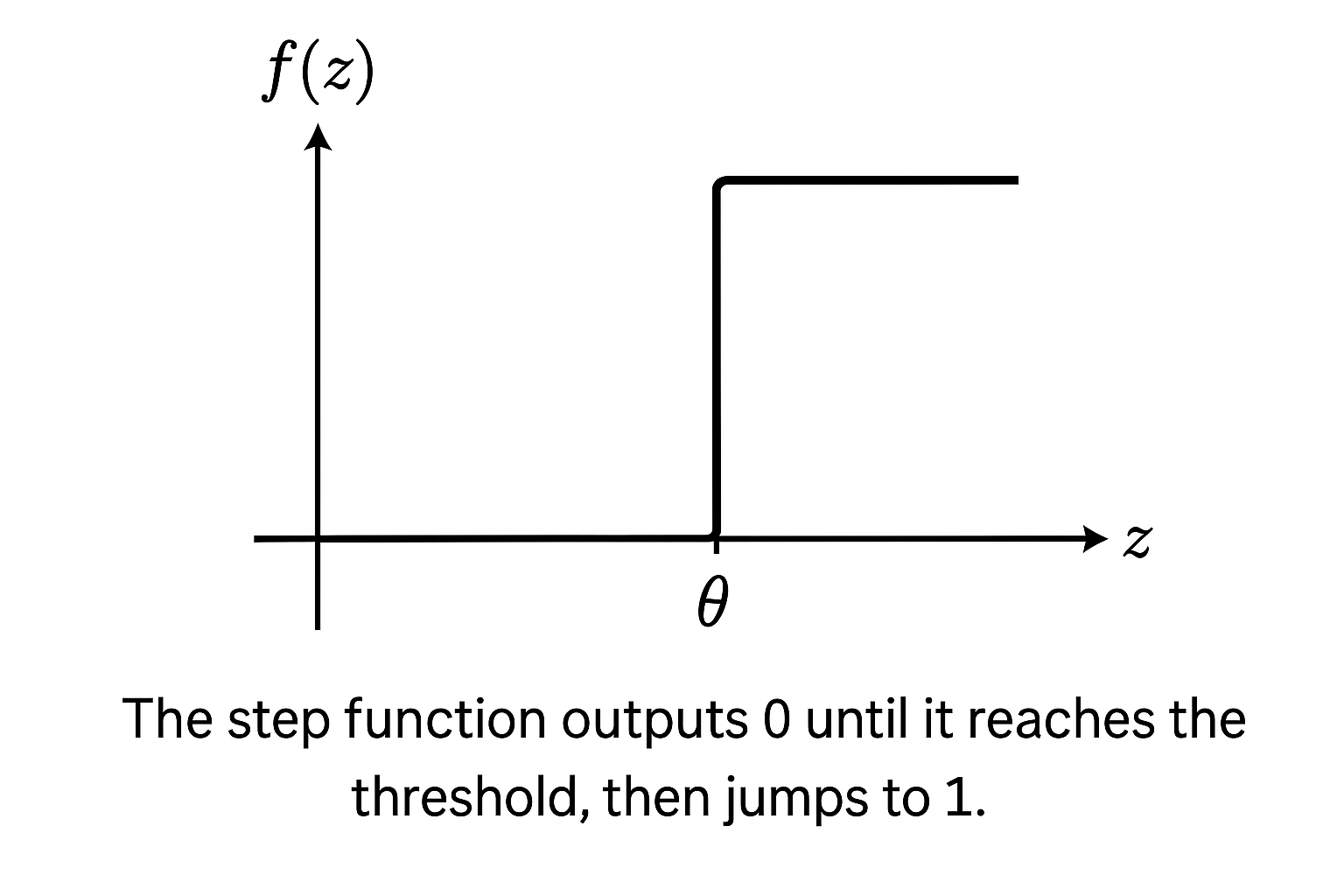
It outputs either 0 or 1 based on whether the combined input crosses a threshold — fine for binary decisions on linearly separable data. The problem is threefold: no gradient to learn from, a sharp discontinuous switch between classifications, and no ability to represent anything beyond straight-line boundaries.
Researchers replaced it quickly with smoother, differentiable functions that could actually support training across multiple layers. The rest of this post covers what they landed on, and why some held up better than others.
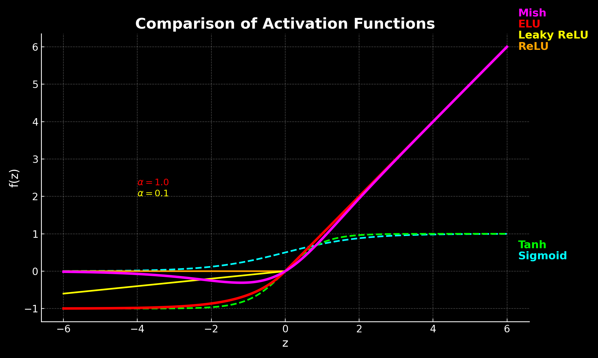
Common activation functions
Each of the following functions was developed to address limitations in whatever came before it. Reading them in order makes the evolution obvious — each one is a direct response to a specific failure mode.
Sigmoid
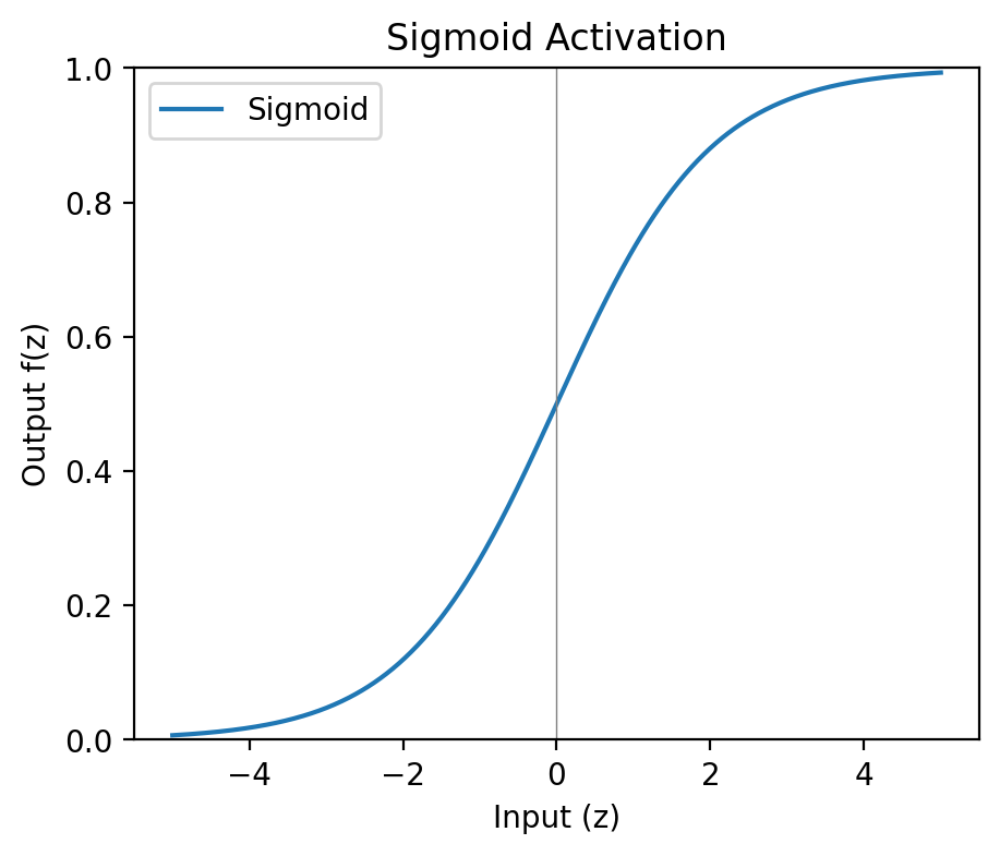
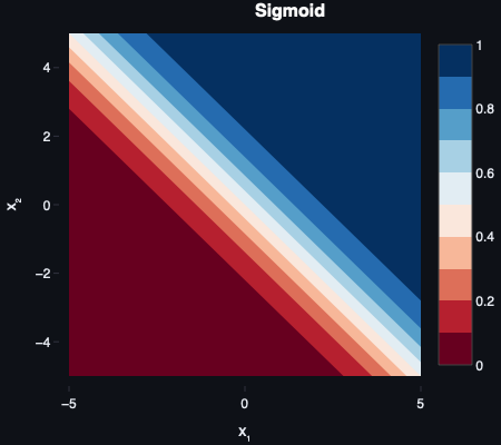
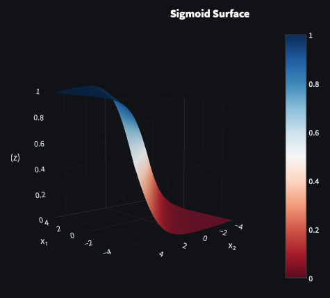
Sigmoid was the natural successor to the step function. Instead of a hard jump from 0 to 1, it produces a smooth curve — small inputs approach 0, large inputs saturate near 1, and there’s a gradual transition between extremes. The fact that outputs fall between 0 and 1 makes them directly interpretable as probabilities — which earns sigmoid its place in output layers.
The problem is what happens at the extremes. When inputs are very large or very small, the curve flattens — the gradient approaches zero. Multiply near-zero gradients across many layers during backpropagation and earlier layers stop learning altogether. That’s the vanishing gradient problem.
In machine learning, a gradient measures how much a function’s output changes when its input changes — the slope of the curve at a given point. During training, gradients tell the network which direction to nudge each weight in order to reduce error. If a gradient is near zero, that weight barely updates regardless of how wrong the output is.
In deep networks, activation functions like sigmoid and tanh produce gradients very close to zero at extreme input values. As these small gradients are multiplied back through many layers during training, they shrink further — eventually so small that early layers stop receiving meaningful updates.
Sigmoid also suffers from not being zero-centred: all outputs are positive, which creates a systematic bias in subsequent layers and slows convergence. For these reasons it’s mostly confined to output layers today, where the probability interpretation earns its keep.
A zero-centred activation outputs values roughly balanced between negative and positive. This helps during optimisation: when activations are centred around zero, gradients can flow in both directions, leading to faster and more stable convergence. Sigmoid’s all-positive outputs create a bias in subsequent layers that slows training down.
Sigmoid became popular in the 1980s alongside backpropagation, notably in Rumelhart, Hinton, and Williams’ Learning Representations by Back‑propagating Errors (1986).
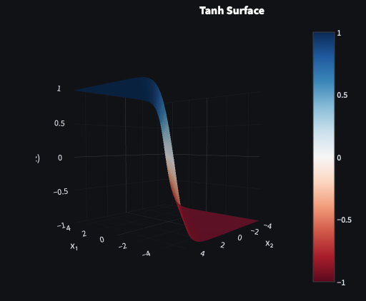
Tanh
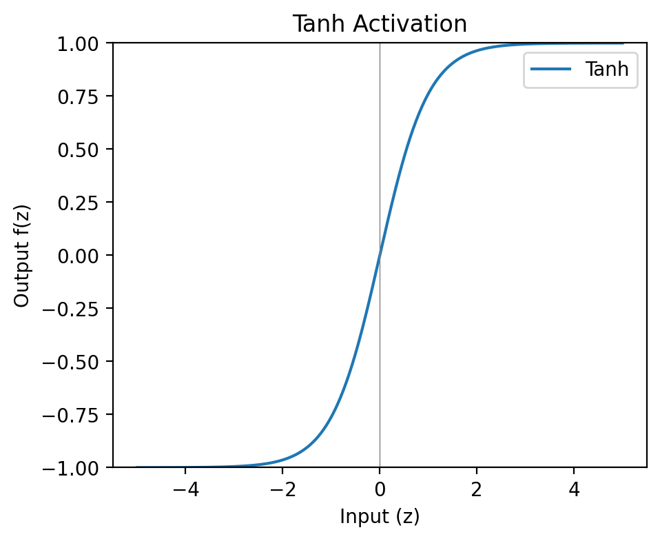
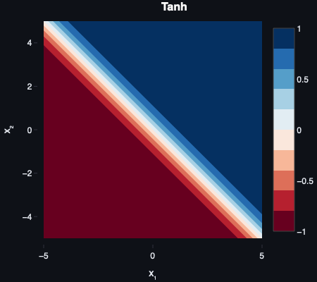
Tanh is sigmoid with the zero-centring problem fixed. Outputs range from -1 to 1 rather than 0 to 1, meaning activations are balanced around zero and gradients can flow in both directions. For shallow networks, it’s a meaningful improvement over sigmoid.
It still saturates at the extremes though — the same vanishing gradient problem lurks at large positive and negative inputs. For deep networks this remains a problem. Tanh held on in recurrent neural networks (RNNs) for longer than it did in feedforward architectures, where its zero-centred outputs were worth the trade-off.
Tanh was popularised as an alternative to sigmoid by Yann LeCun and colleagues in Efficient BackProp (1998).
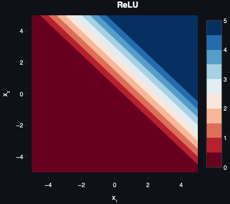
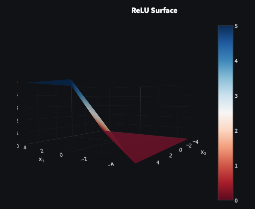
ReLU
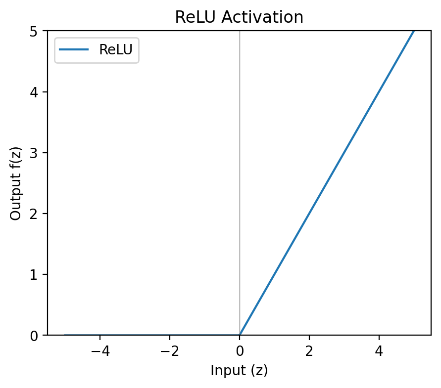
The Rectified Linear Unit (ReLU) is almost aggressively simple — negative inputs are blocked, positive inputs pass through unchanged. No exponential operations, no saturation for positive values, computationally cheap to evaluate and differentiate. In deeper networks the speed advantage compounds significantly.
The catch is the dying ReLU problem. If a neuron’s weights are updated such that all its inputs become negative, it outputs zero permanently. Zero gradient, no further updates. The neuron is effectively dead and never recovers. In large networks a proportion of neurons dying is manageable; in smaller ones it can meaningfully degrade performance.
ReLU gained prominence after Nair and Hinton’s Rectified Linear Units Improve Restricted Boltzmann Machines (2010) and was popularised by Krizhevsky et al. in AlexNet (2012).
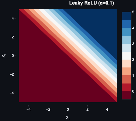
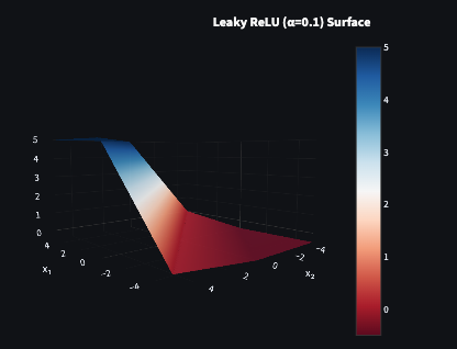
Leaky ReLU
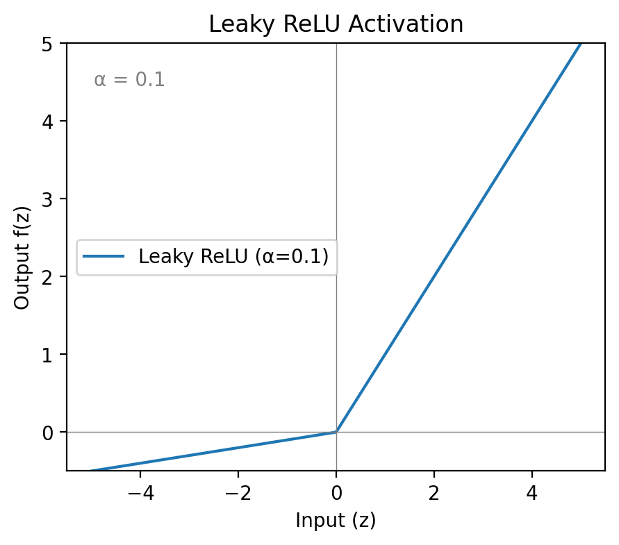
This is the one I’d reach for. Leaky ReLU takes the dying ReLU problem and sidesteps it with one small change: instead of outputting zero for negative inputs, it outputs a small negative value controlled by a hyperparameter — typically 0.01.
A hyperparameter is a value set before training begins — not learned from data, but chosen by the practitioner and tuned against validation performance. in Leaky ReLU controls how much signal passes through on the negative side. The default of 0.01 works well in most cases.
Because negative inputs now produce non-zero outputs, their weights still receive gradients during backpropagation. Neurons can’t die. The computational cost is essentially the same as ReLU — one multiply on the negative path — and mean activations sit closer to zero than standard ReLU, which helps gradient flow in deeper layers.
The only addition is as a hyperparameter to tune, which is a very small price. For most hidden-layer work in feedforward and convolutional networks, Leaky ReLU hits the right balance: fast, stable, and resistant to the failure mode that makes ReLU unreliable.
Leaky ReLU was introduced by Maas et al. in Rectifier Nonlinearities Improve Neural Network Acoustic Models (2013).
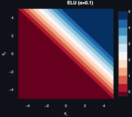
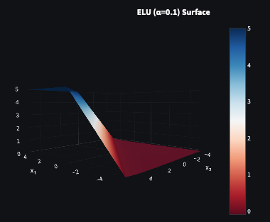
ELU
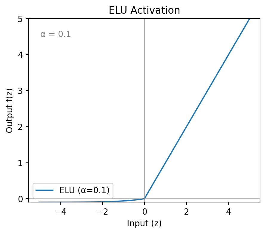
The Exponential Linear Unit takes a similar approach to Leaky ReLU but smooths the negative side with an exponential curve rather than a straight line. The smooth transition pushes mean activations closer to zero and can stabilise training in very deep networks where even small biases compound over many layers.
The exponential on the negative side is more expensive to compute than Leaky ReLU’s simple multiply. It also still requires tuning , and for very negative inputs the exponential approaches zero — so vanishing gradients can still appear at extremes, just less aggressively than with sigmoid or tanh.
ELU makes sense when convergence stability matters more than raw training speed — deep networks where a slightly smoother optimisation curve is worth the compute overhead.
ELU was proposed by Clevert et al. in Fast and Accurate Deep Network Learning by Exponential Linear Units (2015).
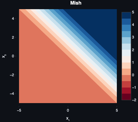
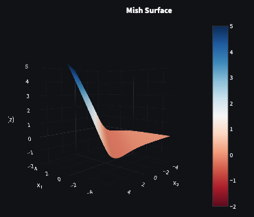
Mish
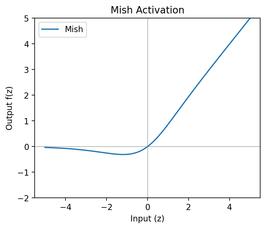
Mish is included for personal reasons, which those of you who know me outside of work will be able to guess at easily enough.
Mish is smooth, non-monotonic, and zero-centred on average. Unlike ReLU and its variants, it dips slightly into negative territory before rising — the curve has a shallow local minimum around — which preserves small negative outputs and has been reported to improve performance in some vision and NLP (Natural Language Processing) tasks. It behaves like a smoother ReLU variant with better gradient flow through the negative region.
The computational overhead is real — the tanh and log operations make it noticeably more expensive than anything in the ReLU family. It’s also relatively new (2019) and less widely supported. Worth experimenting with if the architecture warrants it; not the default choice.
Mish was introduced by Diganta Misra in Mish: A Self Regularized Non-Monotonic Neural Activation Function (2019).
Comparing them side by side
Leaky ReLU and ELU both include a tunable . Common defaults: for Leaky ReLU and for ELU. In Parametric ReLU (PReLU), becomes learnable and is updated during training.
| Function | Output Range | Zero-Centred? | Notes |
|---|---|---|---|
| Step | 0 or 1 | No | Historically important; no gradient — unusable for training. |
| Sigmoid | 0 to 1 | No | Good for output layers where probability interpretation matters. Vanishing gradients make it unsuitable for hidden layers. |
| Tanh | -1 to 1 | Yes | Better than sigmoid in shallow nets; still saturates at extremes. |
| ReLU | 0 to ∞ | No | Fast and effective, but neurons can die permanently on negative inputs. |
| Leaky ReLU | ~-∞ to ∞ | Mostly | Mitigates dying ReLU at near-zero compute cost. My default for hidden layers. |
| ELU | ~-1 to ∞ | Mostly | Smoother negative side improves convergence stability; more expensive than Leaky ReLU. |
| Mish | ~-∞ to ∞ | Mostly | Smooth and non-monotonic; empirically strong in some tasks, computationally expensive, and named after my partner. |
Seeing the difference in practice
Reading about trade-offs is one thing. Here’s a small self-contained experiment: a two-layer network trained on XOR, swapping out the hidden layer activation function and comparing how loss evolves.
XOR is a classic test case because it’s not linearly separable — a single perceptron can’t solve it, but a two-layer network with a non-linear activation can.
import numpy as np
import matplotlib.pyplot as plt

# --- Activation functions and their gradients ---

def sigmoid(z):
    return 1 / (1 + np.exp(-z))

def sigmoid_grad(z):
    s = sigmoid(z)
    return s * (1 - s)

def relu(z):
    return np.maximum(0, z)

def relu_grad(z):
    return (z > 0).astype(float)

def leaky_relu(z, alpha=0.01):
    return np.where(z >= 0, z, alpha * z)

def leaky_relu_grad(z, alpha=0.01):
    return np.where(z >= 0, 1.0, alpha)

# --- XOR dataset ---

X = np.array([[0, 0], [0, 1], [1, 0], [1, 1]], dtype=float)
y = np.array([[0], [1], [1], [0]], dtype=float)

# --- Training loop ---

def train(activation, activation_grad, epochs=5000, lr=0.1, seed=42):
    rng = np.random.default_rng(seed)

    # 2 inputs → 4 hidden units → 1 output
    W1 = rng.standard_normal((2, 4)) * 0.1
    b1 = np.zeros((1, 4))
    W2 = rng.standard_normal((4, 1)) * 0.1
    b2 = np.zeros((1, 1))

    losses = []

    for _ in range(epochs):
        # Forward pass
        z1 = X @ W1 + b1
        a1 = activation(z1)
        z2 = a1 @ W2 + b2
        a2 = sigmoid(z2)  # Output layer uses sigmoid — outputs a probability

        # Binary cross-entropy loss
        loss = -np.mean(
            y * np.log(a2 + 1e-8) + (1 - y) * np.log(1 - a2 + 1e-8)
        )
        losses.append(loss)

        # Backward pass
        dL_da2 = (a2 - y) / len(y)
        dL_dz2 = dL_da2 * sigmoid_grad(z2)

        dL_dW2 = a1.T @ dL_dz2
        dL_db2 = dL_dz2.sum(axis=0, keepdims=True)

        dL_da1 = dL_dz2 @ W2.T
        dL_dz1 = dL_da1 * activation_grad(z1)

        dL_dW1 = X.T @ dL_dz1
        dL_db1 = dL_dz1.sum(axis=0, keepdims=True)

        # Update weights
        W2 -= lr * dL_dW2
        b2 -= lr * dL_db2
        W1 -= lr * dL_dW1
        b1 -= lr * dL_db1

    return losses

# --- Compare activation functions ---

activations = {
    "Sigmoid": (sigmoid, sigmoid_grad),
    "ReLU":    (relu, relu_grad),
    "Leaky ReLU (α=0.01)": (leaky_relu, leaky_relu_grad),
}

fig, ax = plt.subplots(figsize=(10, 5))

for name, (fn, grad_fn) in activations.items():
    losses = train(fn, grad_fn)
    ax.plot(losses, label=name)

ax.set_xlabel("Epoch")
ax.set_ylabel("Loss")
ax.set_title("Training loss on XOR — activation function comparison")
ax.legend()
plt.tight_layout()
plt.savefig("activation_comparison.png", dpi=150)
plt.show()
A few things worth noting in this output:
Sigmoid converges but slowly — the flat regions of the curve mean gradients are small from the start, and on a four-unit hidden layer with a small dataset the effect is visible immediately.
ReLU is faster in early epochs but erratic. On a network this small the dying ReLU problem is observable if you run multiple seeds — occasionally a hidden unit locks to zero and stays there, which shows up as the loss curve plateauing unexpectedly.
Leaky ReLU is consistently the smoothest. Same speed advantage as ReLU without the instability. On this toy problem the difference is modest; on deeper networks or awkward weight initialisations the gap widens.
The point isn’t that one function always wins — it’s that the choice has a measurable effect, and Leaky ReLU’s consistency across conditions is what makes it a reasonable default.
Conclusion
The step function was the right starting point for Rosenblatt — it was simple, binary, and sufficient for linearly separable problems. What it couldn’t do was scale. No gradient means no learning across layers, and no nuance means no complex decision boundaries. Everything that came after it was an attempt to fix one or both of those problems.
Sigmoid fixed the gradient issue but introduced saturation. Tanh fixed the zero-centring problem but kept the saturation. ReLU sidestepped saturation entirely and was fast enough to make deep networks practical — but introduced a new failure mode in neurons that could die permanently. Leaky ReLU addressed that at near-zero additional cost. ELU smoothed the negative side further at the expense of compute. Mish pushed the idea further still.
If someone asked me which to reach for today, the answer is Leaky ReLU for hidden layers and sigmoid for output layers where a probability interpretation is needed. That covers the vast majority of cases. ELU is worth trying when convergence stability is a genuine concern on very deep architectures. Mish is worth knowing about.
With activation functions covered, the series can move on to multilayer perceptrons — how stacking layers with non-linear activations between them produces networks capable of modelling complex relationships. The groundwork is now in place.
Further Reading:
- Perceptrons — the previous post in this series
- Learning Representations by Back-propagating Errors — Rumelhart, Hinton, Williams (1986)
- Efficient BackProp — LeCun et al. (1998)
- Rectified Linear Units Improve Restricted Boltzmann Machines — Nair and Hinton (2010)
- Fast and Accurate Deep Network Learning by Exponential Linear Units — Clevert et al. (2015)
- Mish: A Self Regularized Non-Monotonic Neural Activation Function — Misra (2019)
Part 2 of 3 in Foundations of AI