Perceptrons

Part 1 of 3 in Foundations of AI
Introduction
When I sat down to write this series, I had three reasons that kept pointing in the same direction.
The first was the degree. I wrapped up a part-time undergraduate module on AI and machine learning alongside full-time work, and I found that writing about something is a different kind of understanding to passing an exam on it. The second was clients. I’ve spent a lot of time recently in conversations where people are deploying AI tools they don’t fully understand, and there’s a gap between “this produces useful output” and “I know what’s happening inside it”. The third was the general noise. There’s no shortage of hot takes about AI, but there’s a shortage of explanations that treat a senior software engineer as someone who can handle the mechanics without a PhD.
So this series starts at the bottom. Not because the bottom is where most people are stuck, but because you can’t really understand attention mechanisms or diffusion models without knowing why a perceptron exists. And you can’t know why a perceptron exists without understanding what it was trying to solve.
In 1958, Frank Rosenblatt built a machine that could learn. Not from explicit instructions, but from examples. The original paper is worth a read if you want the historical context. The machine was physical — weights were potentiometers, not floating point values — but the idea it embodied is the one everything else in modern AI is built on: a single unit that takes inputs, applies weights, and fires a decision.
This post unpacks what that actually means, precisely enough that you could implement one yourself.
The goal
By the end of this article, you’ll understand:
- What linear separability means and why it determines what a perceptron can learn.
- How a perceptron processes inputs using weights, bias, and a weighted sum.
- How the step activation function produces a binary decision.
- How the perceptron learning rule adjusts weights from examples.
- Why XOR breaks a single perceptron — and why that matters for everything that comes after.
Prerequisites
- Basic Python (the code example uses NumPy).
- No prior ML knowledge assumed.
What linear separability means
Before opening up the perceptron, it helps to understand the class of problems it was designed to solve. A perceptron is a linear classifier — it draws a straight line. So the question is: which problems can a straight line solve?
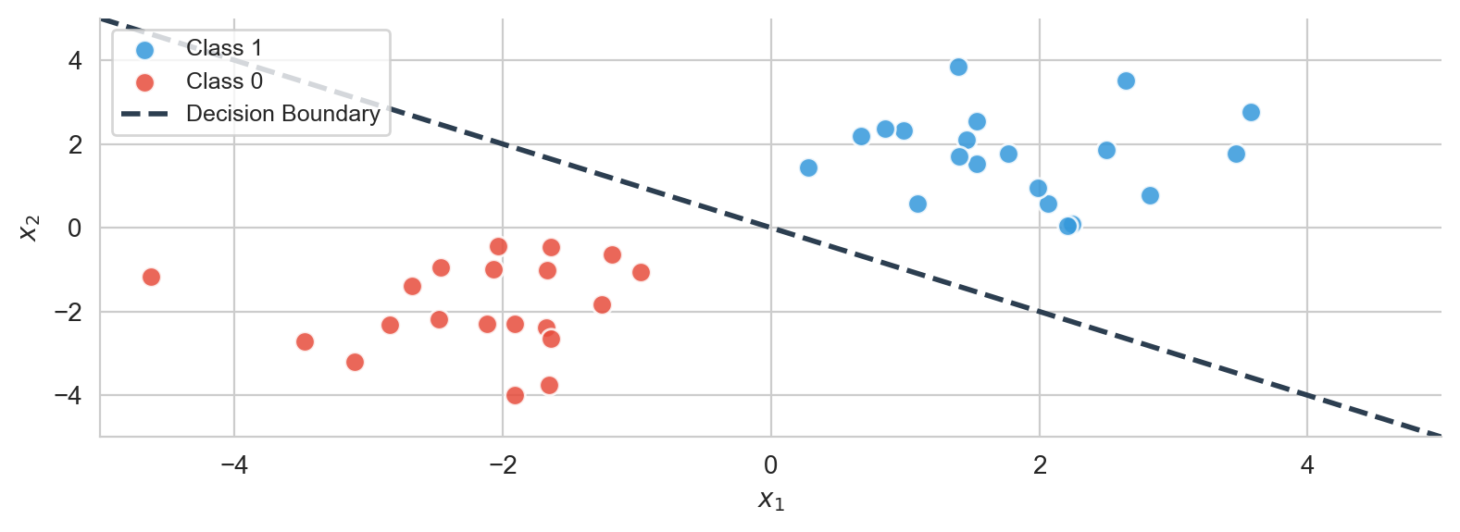
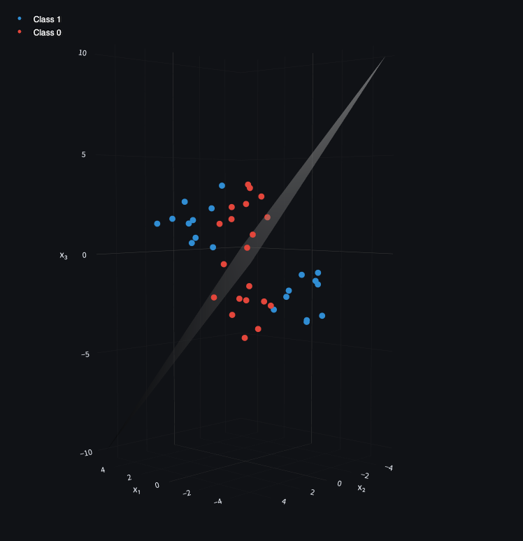
Data is linearly separable if you can draw a straight line (in 2D), a plane (in 3D), or a hyperplane (in higher dimensions) that perfectly divides two classes of points. Everything on one side belongs to Class A; everything on the other belongs to Class B.
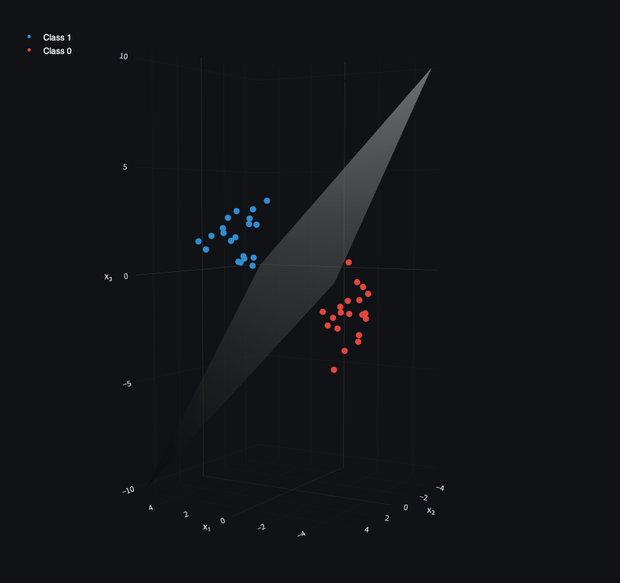
In 3D, the same idea holds — the separator becomes a plane rather than a line.
A class is a label. The category a data point belongs to. Spam vs not-spam, fruit vs vegetable, on vs off. Perceptrons handle binary classification — every point is either Class A or Class B.
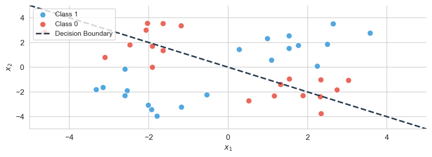
Not all data is linearly separable. The classic counterexample is XOR, which I’ll come back to. For now, understanding linear separability is enough to understand what the perceptron can do — and what it can’t.
Rosenblatt’s 1958 paper didn’t use terms like “linearly separable” or “decision boundary”. Minsky and Papert formalised the limitation in Perceptrons (1969).
Why XOR breaks it
Not all data is linearly separable. Consider exclusive or (XOR):
- If one input is on (1) and the other is off (0), the output is 1.
- If both are on or both are off, the output is 0.
| Input A | Input B | Output |
|---|---|---|
| 0 | 0 | 0 |
| 0 | 1 | 1 |
| 1 | 0 | 1 |
| 1 | 1 | 0 |
Plot the 1s and 0s and they sit in opposite corners — no single straight line separates them.
Minsky and Papert proved this formally in 1969, and the proof contributed to a decade-long slowdown in neural network research. The fix — stacking layers — didn’t get traction until backpropagation was popularised in the 1980s. That’s covered later in this series.
XOR comes up a lot in ML education because it’s the simplest example of a non-linearly separable problem. Any electronics engineer will recognise it as a fundamental gate for binary addition. In practice, the same structure appears wherever two mutually exclusive inputs both push toward the same outcome — you can have one, the other, but not both.
The XOR limitation is what motivates multi-layer networks. A single perceptron can’t solve it; two layers can. That’s the subject of a later post in this series.
Perceptron structure
With linear separability established, here’s what a perceptron actually is.
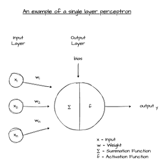
A perceptron is a linear classifier. It maps a vector of input features to a binary output by computing a weighted sum of those inputs, adding a bias, and passing the result through a threshold function. Inputs, weights, bias — then a decision.
Inputs, weights, and bias
Inputs are the numeric values the perceptron considers. Weights are the perceptron’s own view of which inputs matter most — a high weight on an input means that input has more influence over the decision. Bias is an additional learned value that shifts the overall result up or down, independently of the inputs.
All ML operates on numbers. Images, text, audio — everything gets converted into vectors of numeric values before any computation happens.
For a concrete example: say the perceptron is deciding whether to eat a cheesecake or a sticky toffee pudding. Each option is represented as a vector of pixel values (one RGB channel per pixel):
cheesecake = [24, 245, 235, 133, 147, 89, 123, 168, 1,
              178, 34, 103, 64, 165, 157, 92, 52, 30,
              57, 150, 228, 95, 220, 229, 36, 19, 16]

sticky_toffee_pudding = [131, 190, 14, 119, 48, 105, 43, 64, 140,
                         251, 130, 77, 17, 179, 239, 15, 113, 48,
                         149, 26, 133, 244, 151, 108, 30, 24, 69]
Each input has a corresponding weight — how much the perceptron cares about that pixel:
weights = [6, 0, 0, 8, 9, 3, 4, 5, 4,
           9, 1, 3, 9, 10, 5, 6, 3, 7,
           0, 7, 6, 9, 5, 7, 8, 8, 7]
And a bias that shifts the overall result. Since I’d rather have sticky toffee pudding by default, a negative bias pushes the decision toward 0 (sticky toffee pudding) unless the inputs strongly favour cheesecake:
bias = -10The dot product
The core computation of a perceptron is a dot product between inputs and weights. A dot product multiplies two vectors element-by-element and sums the results:
For example:
The dot product projects inputs and weights into a single score. That score, combined with the bias, is what the activation function receives.
GPU prices have tracked AI adoption for a reason. GPUs were originally designed for graphics — and graphics are matrices. A display is rows and columns of pixels, each a vector of RGB values, all updated in parallel. The same matrix arithmetic underpins neural networks, which is why GPUs run AI training so efficiently. The hardware was already purpose-built for it.
The weighted sum
Add the bias to the dot product and you get the perceptron’s pre-activation score:
Where is the weight vector, is the input vector, and is the bias.
The step activation function
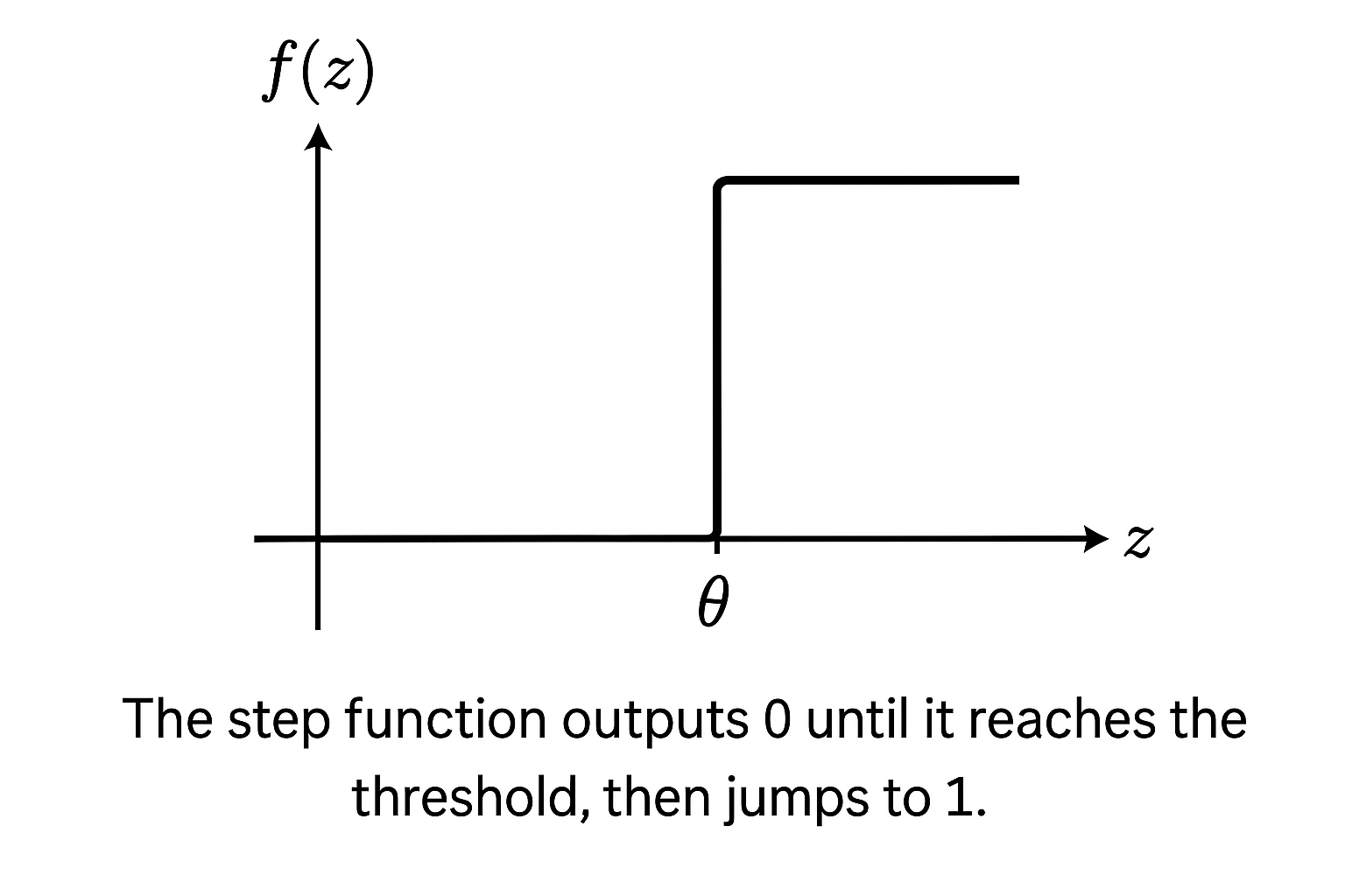
The pre-activation score needs to become a binary decision. The step function does that:
If crosses the threshold , the perceptron outputs 1. Otherwise, 0. The output steps from one to the other at that threshold — hence the name.
This is how the perceptron draws a line. The threshold determines where the decision boundary sits; the weights determine the orientation of the boundary relative to the input space.
The step function works for linearly separable binary classification. For anything else — gradients, multi-class outputs, deep networks — it falls apart immediately. It has no gradient, so there’s no way to train through it in a multi-layer setting. Subsequent activation functions (sigmoid, ReLU, and the rest) were all developed to address that limitation. That’s covered in the next post.
How a perceptron learns
So far, the perceptron has fixed weights. How does it learn them from data?
Rosenblatt’s learning rule is straightforward: for each training example, if the perceptron is wrong, nudge the weights toward the correct answer. The size of each nudge is controlled by a learning rate .
Where:
- = learning rate
- = true label
- = predicted label
- = input value
If the prediction is correct, and the weights don’t change. If the perceptron predicted 0 but the answer was 1, the weights on every input that contributed to the prediction increase. If it predicted 1 and the answer was 0, they decrease. Over many iterations, this shifts the decision boundary into the right position.
This rule is a precursor to backpropagation — not the same thing. It only works for a single layer with a step activation. Backpropagation, which trains multi-layer networks with differentiable activations, is covered later in this series.
Training a perceptron from scratch
Here’s a complete implementation in NumPy. It trains on OR — a linearly separable problem — using the learning rule above.
import numpy as np

def step(z):
    return 1 if z >= 0 else 0

class Perceptron:
    def __init__(self, n_inputs, lr=0.1):
        rng = np.random.default_rng(42)
        self.weights = rng.standard_normal(n_inputs) * 0.01
        self.bias = 0.0
        self.lr = lr

    def predict(self, x):
        return step(np.dot(self.weights, x) + self.bias)

    def train(self, X, y, epochs=10):
        for epoch in range(epochs):
            errors = 0
            for xi, yi in zip(X, y):
                pred = self.predict(xi)
                delta = self.lr * (yi - pred)
                self.weights += delta * xi
                self.bias += delta
                if delta != 0:
                    errors += 1
            print(f"Epoch {epoch + 1}: {errors} error(s)")

# OR dataset — linearly separable
X = np.array([[0, 0], [0, 1], [1, 0], [1, 1]], dtype=float)
y = np.array([0, 1, 1, 1])

p = Perceptron(n_inputs=2)
p.train(X, y, epochs=10)

print("\nFinal predictions:")
for xi in X:
    print(f"  {xi.astype(int)} → {p.predict(xi)}")
Running this produces something like:
Epoch 1: 2 error(s)
Epoch 2: 1 error(s)
Epoch 3: 0 error(s)
Epoch 4: 0 error(s)
...

Final predictions:
  [0 0] → 0
  [0 1] → 1
  [1 0] → 1
  [1 1] → 1
The error count drops to zero within a few epochs and stays there. The perceptron has learned the OR function from examples, without those examples being encoded in any explicit rule.
A few things worth noting. The learning only fires when the perceptron is wrong — delta is zero for correct predictions, so weights only move on mistakes. The bias updates by delta without being scaled by an input; it shifts the decision boundary independently of the input direction. And the whole thing converges because OR is linearly separable. Run the same code on XOR and it never converges — errors keep bouncing. The learning rule can’t find a solution that doesn’t exist.
Conclusion
A perceptron is a weighted sum plus a threshold. Inputs get multiplied by weights, the bias shifts the result, and the step function turns it into a 0 or 1. The learning rule adjusts the weights after each mistake until the decision boundary lands in the right place.
That’s the whole model. One neuron, one line, one binary output.
What Rosenblatt built in 1958 isn’t directly useful for the problems people reach for ML to solve today. But the structure — inputs, weights, a dot product, an activation, a learning signal — is present in every neural network that came after it. The architecture scaled from one neuron to billions; the underlying operation didn’t change.
The limitation is linear separability. Anything a straight line can separate, a perceptron can learn. Anything it can’t — XOR, spiral-shaped data, anything with curves and corners in the decision boundary — requires something more. The next post covers what happens when you introduce non-linear activation functions, which is the first step toward networks that can handle the harder problems.
Further Reading:
- Activation Functions — the next post in this series
- The Perceptron: A Probabilistic Model for Information Storage and Organisation in the Brain — Rosenblatt (1958)
- Perceptrons — Minsky and Papert (1969) — the proof of XOR’s unsolvability by single-layer networks
Part 1 of 3 in Foundations of AI